Reinforcement Learning — Finite Markov Decision Processes (MDP)

MDPs are a classical formalization of sequential decision making, where actions influence not just immediate rewards, but also subsequent situations, or states, and through those future rewards. Thus MDPs involve delayed reward and the need to tradeoff immediate and delayed reward. Whereas in bandit problems we estimated the value $q_*(a)$ of each action $a$, in MDPs we estimate the value $q_*(s, a)$ of each action $a$ in each state s, or we estimate the value $v_*(s)$ of each state given optimal action selections. These state-dependent quantities are essential to accurately assigning credit for long-term consequences to individual action selections.

MDPs are a mathematically idealized form of the reinforcement learning problem for which precise theoretical statements can be made. The key elements of the problem’s mathematical structure, such as returns, value functions, and Bellman equations.

The Agent — Environment Interface

MDPs are meant to be a straightforward framing of the problem of learning from interaction to achieve a goal. The learner and decision maker is called the agent. The thing it interacts with, comprising everything outside the agent, is called the environment. The agent selecting actions and the environment responding to these actions and presenting new situations to the agent. The environment also gives rise to rewards, special numerical values that the agent seeks to maximize over time through its choice of actions.

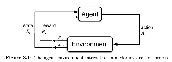
The agent and environment interact at each of a sequence of discrete time steps, $t = 0, 1, 2, 3, …$ .

At each time step $t$, the agent receives some representation of the environment’s state, $S_t \in \mathcal{S}$, and on that basis selects an $action$, $A_t \in \mathcal{A(s)^3}$.

One time step later, in part as a consequence of its action, the agent receives a numerical $reward$, $R_{t+1} \in \mathcal{R} \subset \mathbb R$, and finds itself in a new state, $S_{t+1}$.

The MDP and agent together thereby give rise to a sequence or $trajectory$ that begins like this:

$$ S_0, A_0, R_1, S_1, A_1,R_2,S_2,A_2, R_3, … $$

In a $finite$ MDP, the sets of states, actions, and rewards ($\mathcal{S}, \mathcal{A}, and \ \mathcal{R}$) all have a finite number of elements.

In this case, the random variables $R_t$ and $S_t$ have well defined discrete probability distributions dependent only on the preceding state and action. For particular values of those random variables, $s’ \in \mathcal {S}$ and $r \in \mathcal {R}$, there is a probability of those values occurring at time $t$, given particular values of the preceding state and action: $$ p(s', r|s, a) \doteq Pr\{S_t = s', R_t = r | S_{t-1} = s, A_{t-1} = a \} $$

for all $s’, s \in \mathcal{S}, r \in \mathcal{R}$, and $a \in \mathcal{A(s)}$. The function $p$ defines the $dynamics$ of the MDP. The dot over the equals sign in the equation reminds us that it is a definition (in this case of the function $p$) rather than a fact that follows from previous definitions. The dynamics function $p$: $\mathcal {S} \times \mathcal{R} \times \mathcal{S} \times \mathcal{A} \rightarrow [0, 1]$ is an ordinary deterministic function of four arguments. The ‘|’ in the middle of it comes from the notation for conditional probability, but here it just reminds us that $p$ specifies a probability distribution for each choice of $s$ and $a$,

$$ \sum_{s'\in \mathcal{S}} \sum_{r \in \mathcal{R}} p(s', r|s, a) = 1, \text{ for all }s \in \mathcal {S}, a \in \mathcal {A(s)} $$

In a Markov decision process, the probabilities give by $p$ completely characterize the environment’s dynamics. The probability of each possible value for $S_t$ and $R_t$ depends only on the the immediately preceding state and action, $S_{t-1}$ and $A_{t - 1}$, and given them, not at all on earlier states and actions.

This is best viewed a restriction not on the decision process, but on the $state$. The state must include information about all aspects of the past agent-environment interaction that make a difference for the future. If it does, then the state is said to have the Markov property.

From the four-argument dynamics function $p$, one can compute anything else one might want to know about the environment, such as the $\text{state-transition probabilities}$ (which we denote, with a slight abuse of notation, as a three-argument function $p$: $\mathcal{S} \times \mathcal{S} \times \mathcal{A} \rightarrow [0, 1]$), $$ p(s'|s, a) \doteq Pr\{ S_t = s' | S_{t-1} = s, A_{t - 1} = a\} = \sum_{r \in \mathcal{R}} p(s', r | s, a). $$ We can also compute the expected rewards for state-action pairs as a two-argument function $r$: $\mathcal {S} \times \mathcal {A} \rightarrow \mathbb{R}$: $$ r(s, a) \doteq \mathbb E[R_t|S_{t-1} = s, A_{t-1} = a] = \sum_{r \in \mathcal {}R} r \sum_{s'\in \mathcal{S}}p(s', r|s, a), $$ and the expected rewards for state-action-next-state triples as a three-argument function $r$: $\mathcal {S} \times \mathcal {A} \times \mathcal{S} \rightarrow \mathbb R$, $$ r(s, a, s') \doteq \mathbb E[R_t | S_{t-1} = s, A_{t-1} = a, S_t=s'] = \sum_{r \in \mathcal {R}}r \frac {p(s', r|s, a)} {p(s'|s, a)} $$ The MDP framework is a considerable abstraction of the problem of goal-directed learning from interaction. It proposes that whatever the details of the sensory, memory, and control apparatus, and whatever objective one is trying to achieve, any problem of learning goal-directed behavior can be reduced to three signals passing back and forth between an agent and its environment:

One signal to represent the choices made by the agent (the actions);

One signal to represent the basis on which the choices are made (the states);

One signal to define the agent’s goal (the rewards);

This framework may not be sufficient to represent all decision-learning problems usefully, but it has proved to be widely useful and applicable.

Goals and Rewards

In reinforcement learning, the purpose or goal of the agent is formalized in terms of a special signal, called the reward, passing from the environment to the agent. At each time step, the reward is a simple number, $R_t \in \mathbb R$. The agent’s goal is to maximize the total amount of reward it receives. The agent always learns to maximize its reward. If we want it to do something for us, we must provide rewards to it in such a way that in maximizing them the agent will also achieve our goals. It is thus critical that the rewards we set up truly indicate what we want accomplished. In particular, the reward signal is not the place to impart to the agent prior knowledge about how to achieve what we want it to do.

Returns and Episodes

The agent’s goals is to maximize the cumulative reward it receives in the long run.

The sequence of rewards received after time step $t$ is denoted $R_{t+1}, R_{t+2}, R_{t+3}, …,$ we seek to maximize the expected return, where the return, denoted $G_t$, is defined as. some specific function of the reward sequence,

In the simplest case the return is the sum of the rewards:

$$ G_t \doteq R_{t+1} + R_{t+2} + R_{t+3} + … + R_T $$

where $T$ is a final time step. This approach makes sense in applications in which there is a natural notion of final time step, when the agent-environment interaction breaks naturally into subsequences, which we call episodes. Each episode ends in a special state called the terminal state, followed by a reset to a standard starting state or to a sample from a standard distribution of starting states. Tasks with episodes of this kind are called episodic tasks. In episodic tasks we sometimes need to distinguish the set of all nonterminal states, denoted $\mathcal S$, from the set of all states plus the terminal state, denoted $\mathcal S^+$. The time of termination, $T$, is a random variable that normally varies from episode to episode.

However, in many cases the agent-environment interaction does not break naturally into identifiable episodes, but goes on continually without limit.

Discounting, this approach, is the agent tries to select actions so that the sum of the discounted rewards it receives over the future is maximized. In particular, it chooses $A_t$ to maximize the expected discounted return:

$$ G_t \doteq R_{t+1} + \gamma R_{t+2} + \gamma^2 R_{t+3} + ... = \sum_{k = 0} ^\infty \gamma^k R_{t+k+1} $$ where $\gamma$ is a parameter, $0 \leq \gamma \leq 1$, called the discount rate.

The discount rate determines the present value of future rewards: A reward received $k$ time steps in the future is worth only $\gamma^{k-1}$ times what it would be worth if it were received immediately. If $\gamma < 1$, the infinite sum in $\sum_{k=0} ^{\infty} \gamma^k R_{t+k+1}$ has a finite value as finite value as long as the reward sequence ${R_k}$ is bounded. If $\gamma = 0$, the agent is “myopic” in being concerned only with maximizing immediate rewards: its objective in this case is to learn how to choose $A_t$ so as to maximize only $R_{t+1}$. If each of the agent’s actions happened to influence only the immediate reward, not future rewards as well, then a myopic agent could maximize by separately maximizing each immediate reward.Acting to maximize immediate reward can reduce access to future rewards so that the return is reduced. As $\gamma$ approaches 1, the return objective takes future rewards into account more strongly; the agent becomes more farsighted.

Returns at successive time steps are related to each other in a way that is important for the theory and algorithms of reinforcement learning: $$ \begin{aligned} G_t &\doteq R_{t+1} + \gamma R_{t+2} + \gamma^2 R_{t+3} + \gamma^3 R_{t+4} + ... \\ &= R_{t+1} + \gamma(R_{t+2} + \gamma R_{t+3} + \gamma^2 R_{t+4} + ...) \\ &= R_{t+1} + \gamma G_{t+1}\end{aligned} $$ Note that this works for all time steps $t < T$, event if termination occurs at $t + 1$, if we define $G_T = 0$. This often makes it easy to compute returns from reward sequences.

Note that although the return $\sum_{k=0} ^\infty \gamma^k R_{t+k+1}$ is a sum of an infinite number of terms, it is still finite if the reward is nonzero and constant — if $\gamma < 1$. If the reward is a constant $+1$, then the return is $G_t = \sum_{k = 0} ^{\infty} \gamma^k = \frac {1} {1 - \gamma}$.

Policies and Value Functions

Almost all reinforcement learning algorithms involve estimating value functions (functions of states or of state-action pairs) that estimate how good it is for the agent to be in a given state.

The notion of “how good” here is defined in terms of future rewards that can be expected. or to be precise, in terms of expected return. The rewards the agent can expect to receive in the future depend on what actions it will take. Value functions are defined with respect to particular ways of acting, called policies.

A policy is a mapping from states to probabilities of selecting each possible action. If the agent is following policy $\pi$ at time $t$, then $\pi(a|s)$ is the probability that $A_t = a$ if $S_t = s$. Like $p$, $\pi$ is an ordinary function; the “$|$” in the middle of $\pi(a|s)$ merely reminds that it defines a probability distribution over $a \in \mathcal A(s)$ for each $s \in \mathcal {S}$.

The value function of a state $s$ under a policy $\pi$, denoted $v_\pi(s)$, is the expected return when starting in $s$ and following $\pi$. For MDPs, we can define $v_\pi$ formally by, $$ v_\pi(s) \doteq \mathbb E_\pi [G_t|S_t = s] = \mathbb E_\pi[\sum_{k = 0} ^\infty \gamma^k R_{t+k+1} | S_t = s], \text{ for all } s \in \mathcal S $$ where $\mathbb E_\pi[\cdot]$ denotes the expected value of a random variable given that the agent follows policy $\pi$, and $t$ is any time step. Note that the value of the terminal state, if any, is always zero. We call the function $v_\pi$ the state-value function for policy $\pi$.

Similarly, we define the value of taking action $a$ in state $s$ under a policy $\pi$, denoted $q_\pi(s, a)$, as the expected return starting from s, taking the action $a$, and thereafter following policy $\pi$:

$$ q_{\pi}(s, a) \doteq \mathbb E_{\pi}[G_t | S_t=s, A_t = a] = \mathbb E_{\pi}[\sum_{k = 0} ^{\infty} \gamma^k R_{t+k+1} | S_t = s, A_t = a] $$

where $q_\pi$ is the action-value function for policy $\pi$.

A fundamental property of value functions used throughout reinforcement learning and dynamic programming. This is their relationship, for any policy $\pi$ and any state $s$, the following consistency condition holds between the value of $s$ and the value of its possible successor states: $$ \begin {aligned} v_{\pi}(s) &\doteq \mathbb E[G_t | S_t = s] \\ &= \mathbb E_{\pi}[R_{t+1} + \gamma G_{t+1} | S_t = s] \\ &=\sum_{a}\pi(a|s) \sum_{s'} \sum_{r} p(s',r|s,a)[r + \gamma \mathbb E[G_{t+1} | S_{t+1} = s']] \\ &=\sum_a \pi(a|s) \sum_{s',r} p(s', r|s, a)[r + \gamma v_{\pi}(s')], \text { for all } s \in \mathcal {S} \end {aligned} $$ where it is implicit that the actions, $a$, are taken from the set $\mathcal A(s)$, that the next states, $s’$, are taken from the set $\mathcal S$, and that the rewards, $r$, are taken from the set $\mathcal R$.

$\sum_{a} \pi(a|s) \sum_{s',r} p(s', r | s, a) [r + \gamma v_\pi(s')]$ is the Bellman equation for $v_\pi$. It expresses a relationship between the value of a state and the values of its successor states.

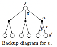
Think of looking ahead from a state to its possible successor states, as suggested by the diagram to the right. Each open circle represents a state and each solid circle represents a state-action pair. Starting from state $s$, the root node at the top, the agent could take any of some set of actions — three are show in the diagram — based on its policy $\pi$. From each of these, the environment could respond with one of several next states, $s’$, along with a reward, $r$, depending on its dynamic given by the function $p$. The Bellman equation averages over all the possibilities, weighting each by its probability of occurring. It states that the value of the start state must equal the value of the expected next state, plus the reward expected along the way.

Above diagrams called backup diagrams, they diagram relationships that form the basis of the update or backup operations that are at the heart of reinforcement learning methods. These operations transfer value information back to a state (or a state-action pair) from its successor states (or state-action pairs).

Optimal Policies and Optimal Value Functions

Solving a reinforcement learning task means, roughly, finding a policy that achieves a lot of reward over the long run. For finite MDPs, we can precisely define an optimal policy in the following way. Value functions define a partial ordering over policies. A policy $\pi$ is defined to be better than or equal to a policy $\pi’$ if its expected return is greater than or equal to that of $\pi’$ for all states.

In other words, $\pi \geq \pi’$ if and only if $v_{\pi} (s) \geq V_{\pi’}(s)$ for all $s \in \mathcal S$. There is always at least one policy that is better than or equal to all other policies. This is an optimal policy. Although there may be more than one, we denote all the optimal policies by $\pi_{}$. They share the same state-value function, called the optimal state-value function, denoted $v_$, and defined as

$$ v_*(s) \doteq \max_\pi V_{\pi}(s),\text{ for all } s \in \mathcal S $$

Optimal policies also share the same optimal action-value function, denoted $q_*$, and defined as

$$ q_*(s, a) \doteq \max_{\pi} q_{\pi}(s, a), \text{ for all } s \in \mathcal S \text{ and } a \in \mathcal A(s). $$

For the state-action pair $(s, a)$, this function gives the expected return for taking action $a$ in state $s$ and thereafter following an optimal policy. Thus, we can write $q_$ in term of $v_$ as follows: $$ q_*(s, a) = \mathbb E[R_{t+1} + \gamma v_*(S_{t+1}) | S_t = s, A_t = a] $$

Optimality and Approximation

An agent learns an optimal policy has done very well, but in practice this rarely happens. For the kinds of tasks in which we are interested, optimal policies can be generated only with extreme computational cost.

The memory available is an important constraint. A large amount of memory is often required to build up approximations of value functions, policies, and models. In tasks with small, finite state sets, it is possible to from these approximations using arrays or tables with one entry for each state (or state-action pair). This we call the tabular case, and the corresponding methods we call tabular methods. In many cases of practical interest, however, there are far more states than could possibly be entries in a table. In these cases the functions must be approximated, using some sort of more compact parameterized function representation.

Summary

Reinforcement learning is about learning from interaction how to behave in order to achieve a goal. The reinforcement learning agent and its environment interact over a sequence of discrete time steps. The specification of their interface defines a particular task: The actions are the choices made by the agent; the states are the basis for making the choices; and the rewards are the basis for evaluating the choices. Everything inside the agent is completely known and controllable by the agent; everything outside is incompletely controllable but may or may not be completely known. A policy is a stochastic rule by which the agent selects actions as a function of states. The agent’s objective is to maximize the amount of reward it receives over time.

When the reinforcement learning setup described above is formulated with well defined transition probabilities it constitutes a Markov Decision Process (MDP). A finite MDP is an MDP with finite state, action, and reward sets. Much of the current theory of reinforcement learning is restricted to finite MDPs, but the methods and ideas apply more generally.

The return is the function of future rewards that the agent seeks to maximize. It has several different definitions depending upon the nature of the task and whether one wishes to discount delayed reward. The un-discounted formulation is appropriate for episodic tasks, in which the agent-environment interaction breaks naturally into episodes; the discounted formulation is appropriate for continuing tasks, in which the interaction does not naturally break into episodes but continues without limit. We try to define the returns for the two kinds of tasks such that one set of equations can apply to both the episodic and continuing cases.

A policy’s value functions assign to each state, or state-action pair, the expected return from that state, or state-action pair, given that the agent uses the policy. The optimal value functions assign to each state, or state-action pair, the largest expected return achievable by any policy. A policy whose value functions are optimal is an optimal policy. Whereas the optimal value functions for states and state-action pairs are unique for a given MDP, there can be many optimal policies. Any policy that is greedy with respect to the optimal value functions must be an optimal policy. The Bellman optimality equations are special consistency conditions that the optimal value functions must satisfy and that can be solved for the optimal value functions, from which an optimal policy can be determined with relative ease.

If the agent has a complete and accurate environment model, the agent is typically unable to perform enough computation per time step to fully use it. The memory available is also an important constraint. Memory may be required to build up accurate approximations of value functions, policies, and models. In most cases of practical interest there are far more states than could possibly be entries in a table, and approximations must be made.

References

1. Sutton, R. S., & Barto, A. G. (2018). Reinforcement learning: An introduction (2nd ed.).